Beta-Binomial Model and Multilevel Binomial Model: A Comparison
One day I was experimenting with these two models, completely unaware they’d turn out to be the same*!
In this blog, I’ll explore an interesting statistical relationship that I came to realize while experimenting with these two models: the Beta-Binomial Model and the Multilevel Binomial Model.
The term “multilevel” can be quite vague when describing these models. For clarity, I have a detailed section on model specification later in this post that will help you understand exactly what I mean by a “multilevel binomial model” in this context.
Quick Intro on Beta-Binomial likelihood
Let us assume the random variable S(success) to be binomially distributed, as
\[S_i|\theta \sim Binomial(n,\theta)\]Note that \(S_i\) is not marginally Binomial; it is conditionally Binomial, given \(\theta\). If \(\theta\) varies across trials then the marginal distribution of S is called the Beta-Binomial distribution. i.e
\[S_i \sim BetaBinomial(n,{\theta})\]Thus, these types of likelihood/ models are widely used to account for dispersion in the data as \(\theta\) varies across trials.
Data
For demonstration purposes, I have simulated only two variables: the Number of Trials (N), which is fixed for each experiment, and the Number of Successes (S).
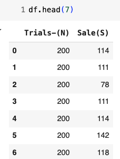
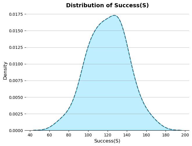
Figure: Data visualization and distribution of the simulated data
Full model Specifications
I have reparameterized both models using the same parameterization and assigned identical priors to ensure a fair comparison. For the Beta-Binomial model, I’ve expressed the parameters \(\alpha\) and \(\beta\) in terms of \(\mu\) (mean) and \(k\) (concentration), where \(\alpha = \mu*k\) and \(\beta = (1-\mu)*k\). These are common reparameterization in these kinds of models as these are easy to interpret.
Beta Binomial (Model 1)
\[S \sim BetaBinomial(n,\alpha,\beta) \quad Model\ 1\] \[\alpha = \mu * k\] \[\beta = (1-\mu)* k\]Multilevel Binomial (Model 2)
\[S_{i} \sim Binomial(n,\theta_{i}) \quad Model\ 2\] \[\theta_i \sim Beta(\alpha,\beta) \quad Prior\] \[\alpha = \mu* k\] \[\beta = (1-\mu)* k\]Prior
To ensure a fair comparison between the two models, we’ll use identical prior distributions for both. This is particularly important for the beta prior on \(\theta\). This approach allows us to isolate the structural differences between the models without introducing bias from different prior specifications.
Priors : Beta Binomial (Model 1)
\[\mu \sim Beta(10,10)\] \[k \sim Exponential(1/10)\]Priors :Multilevel Binomial (Model 2)
\[\mu \sim Beta(10,10)\] \[k \sim Exponential(1/10)\]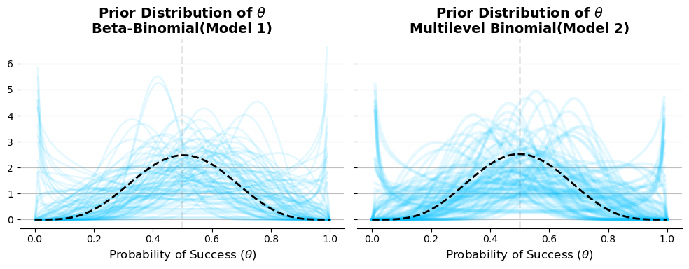
Fig: Prior distribution for probability of success \(\theta\).
As shown in the figure above, we can see that the same prior distributions have been provided for both models. This plot verifies the prior distribution of the probability of success, \(\theta\).
Posterior
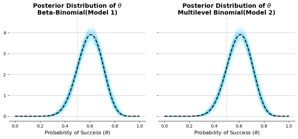
Figure: Posterior Distribution of \(\theta\)
The plot shows that the model produces similar estimates for \(\theta\). This is not a coincidence; rather, it is because the underlying specifications of the models are the same under these assumptions.
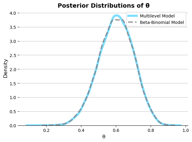
Figure: Posterior Distribution of \(\theta\)
Both models that we tried above produced similar estimates because they handled overdispersion in comparable ways. The multilevel-binomial model accounted for overdispersion by allowing the probability of success to vary across observations through random effects. Similarly, the beta-binomial model handled overdispersion by incorporating variability in the success probability using a beta distribution.
The key difference is that the multilevel binomial model can offer more flexibility and additional tools for modeling overdispersion. This flexibility will allow us to incorporate group-level structures and other hierarchical relationships that might be present in the data, while still accounting for the extra variability that overdispersion introduces.
Choosing the Right Model
All these comparisons boil down to choosing the right model. Choosing the right model depends on several factors. If you only need the overall probability of success, \(\theta\), as used here, the Beta-Binomial model (Model 1) is a good choice because it samples faster than the multilevel model. However, if you are interested in the probability of success for each individual trials, \(\theta_{i}\), you need to use the Multilevel Binomial model (Model 2). Additionally, since Multilevel models allow more flexibility to handle dispersion in the data, they are preferable when you need to account for complex hierarchical structures or when the overdispersion patterns are more nuanced. Below is the plot for the probability of success for the first 5 observations.
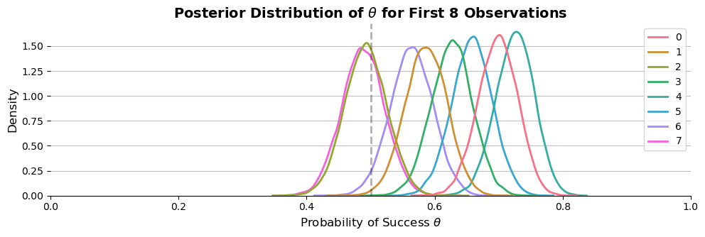
Figure: Posterior Distribution of \(\theta\) for first five trials/experiment
Choosing the right model depends on the research questions at hand. I typically prefer multilevel models whenever I can, as they help understand the data at hand and have other interpretable properties. For example, see Models with memories