Rate of an Event Analysis
Context
Businesses are often interested in knowing the rate at which their customers enroll and quit. It is through these rates that any business decides upon its customer retention strategies and evaluates the lifetime value of each customer.
In this project, we are considering data from a subscription-based e-commerce platform. We are interested in the rate at which customers unsubscribe during the previous two years and compare it with our new strategy.
Understanding such rates is crucial for businesses for mainly two reasons:
- They can further investigate the causes of increased unsubscription rates and improve the system by making the right inferences.
- Such rates help businesses evaluate the lifetime value of each customer, which helps them spend wisely.
Data & Methods
The idea is not just to predict the rate of unsubscription but to prevent it. We then compare the new strategy to the old one based on two years of data on active/inactive users.
- enrolled_date: Date when the customer is enrolled.
- status_unsubscribed: Status of whether the customer is enrolled.
- active_days: Total days when the customer is active.
- new_strategy: Indicator of the new strategy implemented.
Implementation, Assumptions, and Priors
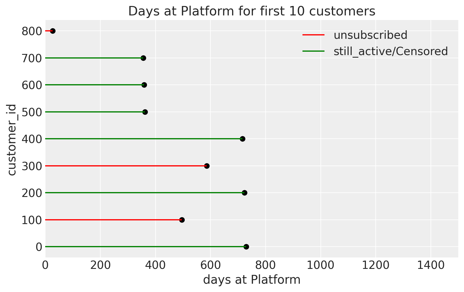
One problem with these types of analyses is that the dataset represents a certain time window. There will be a mix of customers currently continuing and customers who have dropped out in the dataset. This can create confusion as the customers currently continuing their academics will still be in that dataset, but we are interested in only dropout rates. Therefore, an instinct might be to delete data of customers who haven’t dropped out.
However, this is a mistake and can cause biased estimates because the customers who have not dropped out until we download the data give us information about the dropout rate by representing that they haven’t dropped out.
This is confusing, but one loose example to understand this is as simple as: the probability of a head gives us information about the probability of a tail, as they are complementary to each other.
But we cannot still strongly generalize the relationship between performance and incentives. The generalization is important to us because we want to make predictions outside the sample. We do this by testing the fact that inexperienced volunteers will have less effect on their performance despite getting incentives compared to experienced ones from our data. The proxy to experience is captured by our performance metric, but it doesn’t have to be only experience; it can be anything that drives performance.
So, we are implying that there may be a correlation between the intercept and the slopes, which will further help us to squeeze more generalized information out of the data.
Such data are called censored data, and now you could guess why it’s called censored. Survival models are go-to models for such data. Survival analysis has been used for data involving time to a certain event, such as death, the onset of a disease, or other biological events, but we can borrow its applications in business. Here, we will be using a simple version of survival models and using the Exponential Distribution for our likelihood.
About Exponential Distribution
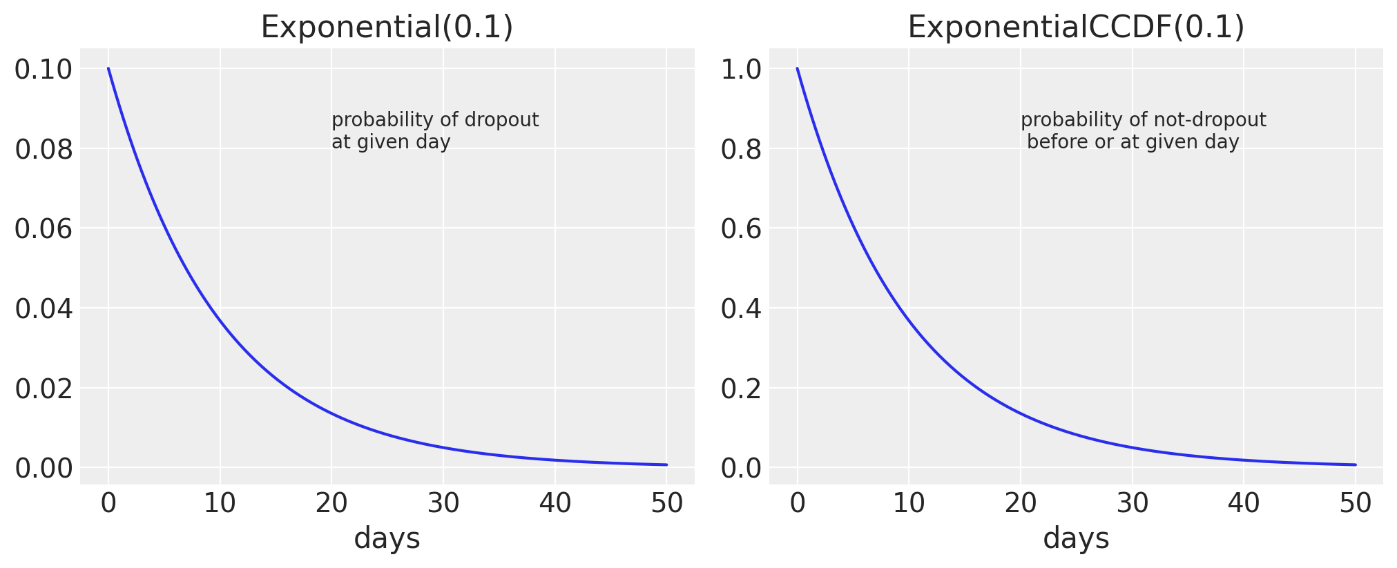
The Exponential Distribution is the probability distribution of the time between events in which such events occur continuously and independently at a constant average rate.
It has only one parameter, \(\lambda\). The \(\lambda\) parameter is the rate of an event happening, which is exactly what we wanted to figure out. Also, the memorylessness feature of the exponential distribution states that every day, each customer has some constant rate of dropping out.
Model
Let,
\(D_{i} = \text{days to event}\)
\(\lambda = \text{unsubscription rate}\)
\(D_{i}|\text{unsub} == 1 \sim \text{Exponential}(\lambda)\)
\(D_{i}|\text{unsub} == 0 \sim \text{Exponential}(\lambda)\)
where;
\(\lambda_{i} = \exp(a[\text{unSub}])\)
For customers who have unsubscribed, their rate is just exponentially distributed as per our assumption. But for customers who have not yet dropped out, we can incorporate their information using the Exponential CCDF, which is just the cumulative complementary of the Exponential Distribution. For example, since a customer has not yet unsubscribed until day 25, it is the probability of not dropping out before or on the 25th day. We can further explore these topics mathematically.
The above notation can be further written as:
\(\begin{cases}
e^{-\lambda t} & \text{if dropout} == 0 \\
\lambda e^{-\lambda t} & \text{if dropout} == 1
\end{cases}\)
Priors
Priors are your beliefs about our parameters before seeing the data. It’s just a way of telling our model what is infinity and what’s not. You can also incorporate your expert beliefs, findings from your previous studies, or even some sensible reasoning about your parameter into your prior.
In this example, we are estimating the dropout rate of each student per day, i.e., the parameter \(\lambda\). Before even seeing the data, we can have some reasoning about this parameter; even though we can’t exactly estimate what value \(\lambda\) can take right now, we know what values it cannot take. For instance, imagine \(\lambda\) is 0.50 or more, i.e., a dropout rate of each student per day is 50% or more; we know for certain that no school can even think of running a successful business with that dropout rate unless it’s into some serious money laundering. Of course, we can do far better than that, but even a simple restriction can improve our model’s estimation because our model does not have to look for impossible infinite space. We want \(\lambda\) to fall under 0.5 and increase our beliefs as we move below.
But our beliefs should be converted into mathematical notation for our model to make sense. Eliciting priors, especially on these kinds of Generalized Linear Models (GLMs), is tricky because we have morphed the parameters using some link function to our GLMs. Therefore, it’s always suggested to plot the priors.
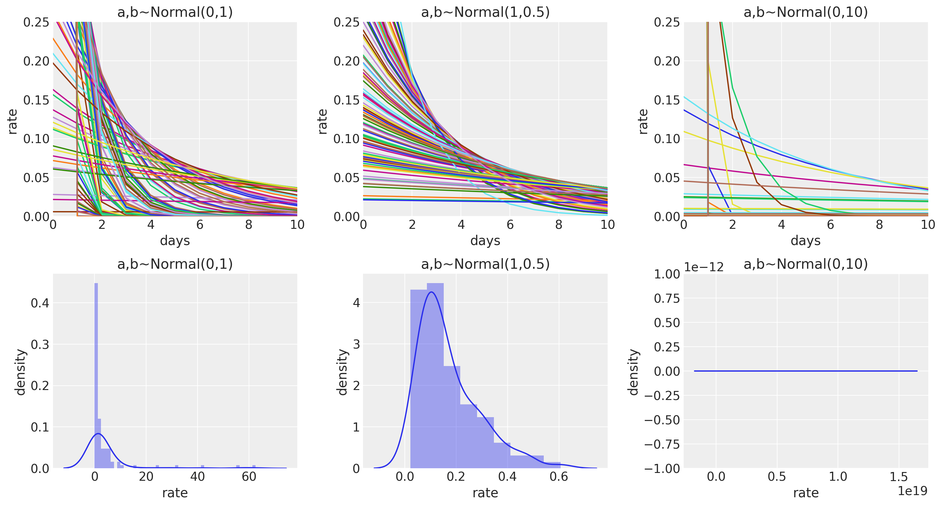
Priors:
\(\alpha \sim \text{Norm}(1, 1.5)\)
\(\beta \sim \text{Norm}(1, 1.5)\)
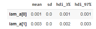
Findings