How Randomization Magically Works ..

One random day, I was having a conversation with someone I’ll call Mike—a Statistics Guru who would soon change how I understood randomization.

I told him about how I use randomization everyday in my work, but honestly, I’d never really grasped how it actually works. All those theory, mathematical notations , assumptions, and terms like exchangeability, just end up clouding my understanding of randomization.

Mike smiled, as if he knew something that I hadn’t, and said,

“Let me make it easy for you. I’ll show you how randomization really works in a simplest way that the world had never seen before.”

Of course that was an overstatement from Mike, but what he showed me was entirely new to me—even though it’s been around since long before computers. All the text books I had read in my curriculum never included this. Then, as if to make things even more intriguing Mike said yet another controversial statement

“We’re going to use simulation to explore randomization. This is how engineers came to understand statistics.”

Simulations? To understand something as theoretical as randomization? It sounded counterintuitive at first but I was intrigued.

Excited and curious, I was ready to dive in. What followed was an insightful, hands-on demonstration that made everything click.

Let me walk you through it step by step, because it changed how I think about randomization forever.

Context

Let’s start with an overused but illustrative research question:

Does drinking coffee cause cancer?

Now, imagine you’re the researcher tasked with estimating this effect and reporting your findings to authorities who might decide to implement a coffee ban if your results suggest a link.

To begin, let’s be naive. Suppose we simply survey people to ask whether they drink coffee frequently and whether they have (or had) cancer. At this stage, we haven’t applied randomization yet. Why not? because before appreciating the importance of randomization, lets first fall into pitfalls of not using it.

From here on, it’s helpful to represent the Variables visually using a DAG (Directed Acyclic Graph); a DAG is a simple way to show relationships between variables: each node represents a variable, and the arrows indicate how they influence one another.

Take a look at this DAG (Fig. 1), which illustrates the data generation process we’ve been discussing.

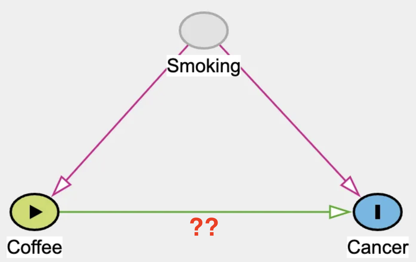
Fig 1: DAG; a without randomization

If you examine this DAG closely, you’ll notice a variable called “Smoking.” While it isn’t the focus of our research question, it plays a critical role in the analysis.People who smoke are more likely to consume beverages like coffee, which is why there’s an arrow connecting Smoking to Coffee. Additionally, we know that smoking increases the risk of cancer, represented by the arrow from Smoking to Cancer. Here’s the catch: when you surveyed people about their coffee consumption, you didn’t ask about their smoking habits. However, in an observational setting, ignoring a variable doesn’t mean its influence disappears.

[Spoiler alert] Coffee doesn’t actually cause cancer and we are going to use this information to simulate our data. However, smokers tend to drink more coffee, and this correlation introduces complications in the analysis.

We’ll explore how the “Smoking” variable significantly affects the results later. For now, let’s move on to simulating the data.

import numpy as np
import pandas as pd
from scipy.special import expit as logistic
n_sample = 200
Smoking = np.random.binomial(1,0.4,size = n_sample)
Coffee = np.random.binomial(1,logistic(-2 + 2.5*Smoking))
Cancer = np.random.binomial(1,logistic(-2 + 2*Smoking + 0*Coffee))

df = pd.DataFrame({
    'Smoking':Smoking,
    'Coffee':Coffee,
    'Cancer':Cancer})

Lets go through these lines of code in sequential order

n_sample = 200

We are generating 200 samples for this case. A typical study might include fewer or more than this. The optimal sample size depends on many factors, which are beyond the scope of this article.

Smoking = np.random.binomial(1,0.4,size = n_sample)

The function np.random.binomial(1, 0.4, size=n_sample) generates a sample where approximately 40% of the participants are smokers.

Coffee = np.random.binomial(1,p=logistic(-2 + 2.5*Smoking))

the proportion of Coffee drinkers, p = logistic(-2 + 2.5*Smoking), depends on Smoking. Logistic is a sigmoid function which just transforms the values into proportion i.e between 0 and 1. So, if Smoking is 0 then the logistic(-2 + 2.5* 0 ) is around 0.12 . and if Smoking is one then logistic(-2 + 2.5* 1) is around 0.62. Thus, the smokers are more likely to be frequent Coffee drinkers than the non-smokers.

Cancer = np.random.binomial(1,logistic(-2 + 2*Smoking + 0*Coffee))

Again, proportion of Cancer p = logistic(-2 + 2Smoking + 0Coffee) , depends on Smoking again and not coffee as 0* Coffee is equal to zero.

Now, Lets store these to Data-frames, note that I have also included Smoking for reference but in reality we have not measured those.

df = pd.DataFrame({'Smoking':Smoking,'Coffee':Coffee,'Cancer':Cancer})

We store these into the data frame.

To revise this, In this simulation:

• The effect of coffee on cancer is set to zero.
• Smoking will be introduced as a confounder, influencing both coffee consumption and cancer risk, but it will not be included in the dataset.

This setup mirrors real-world situations where confounding factors can distort the apparent relationships between variables. Now, let’s fit a logistic regression model to test the relationship between coffee consumption and cancer:

Model 1 : \(`Cancer \sim Coffee`\)

In this model, we are examining how cancer is influenced by coffee consumption. The code below demonstrates how to fit this model. Don’t worry if the details of the code are unclear for now — the focus is on estimating the relationship between coffee and cancer as specified in the model.

import statsmodels.formula.api as smf
# Fit the linear regression model
model = smf.logit('Cancer ~ Coffee', data=df).fit()

# Accessing model parameters using attributes and storing these into datafame
params = pd.DataFrame({
    'Parameter': model.params.index,
    'Estimate': model.params.values,
    'Standard Error': model.bse.values,
})

# Extract the estimate and standard error for Coffee
coffee_estimate = params.loc[params['Parameter'] == 'Coffee', 'Estimate'].values[0]
coffee_se = params.loc[params['Parameter'] == 'Coffee', 'Standard Error'].values[0]

# Calculate the confidence interval
lower_ci = 1.96 * coffee_se
upper_ci = 1.96 * coffee_se
# Create the forest plot
fig,axs  = plt.subplots(figsize=(8, 6))
axs.errorbar(
    x=[coffee_estimate], y=[1],
    xerr=[[lower_ci], [upper_ci]],
    fmt='o', capsize=5,label="Model estimate")
axs.set(yticks = [1],yticklabels = ["Coffee effect \n on Cancer"],
        title ='Model : Cancer ~ Coffee \n Without Randomization',xlim=(-3,3),xlabel ='Effect Estimate',
        ylabel = '',)
axs.axvline(x=0, color='black',
            linestyle='--',alpha = 0.2,
            label="True estimate")
plt.legend()
plt.show()

Figure 2: Parameter Estimates

The observed association between coffee and cancer appears positive, as the estimates (represented by the blue dots) are clearly greater than zero. However, this is not a causal effect. How do we know that? Because, we explicitly set the causal effect of coffee on cancer to zero in our simulation. The true cause of cancer is smoking, which also influences coffee consumption. This creates a positive association between coffee and cancer, but it’s not causal—it’s driven by smoking acting as a confounder that affects both variables.

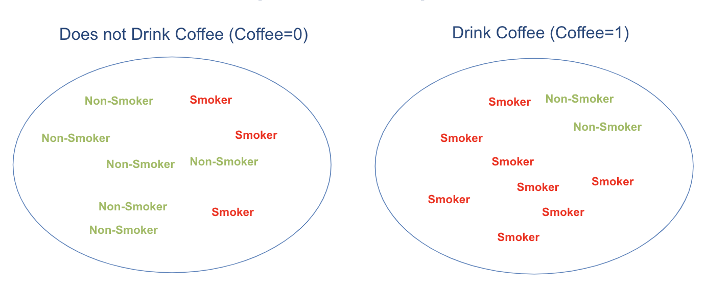
To better understand this, consider an illustration: the proportion of smokers is higher in the coffee-drinking group compared to the non-coffee group. This makes the two groups non-comparable, or more precisely, non-exchangeable.

Introducing Randomization

Now that we understand the limitations of the previous approach, we can better appreciate the crucial role randomization plays.

Consider this new DAG (Figure 3):

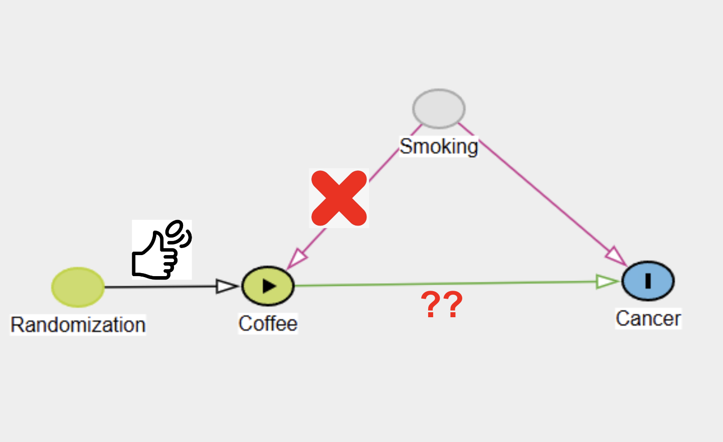
Figure 3 : DAG Randomized

The key difference here is that the arrow from Smoking to Coffee is missing. Instead, we’ve used randomization to assign coffee consumption. This means, for each participant, we flip a coin to assign them to either the Coffee or No-Coffee group, and then track them over time—whether it’s 1, 10, or 30 years—depending on the study’s design. While this process may seem impractical for quickly obtaining results, simulations allow us to “travel through time” and understand how the analysis would unfold, providing valuable insights into the impact of randomization.

# Randomization
n_sample = 200
Smoking = np.random.binomial(1,0.4,size = n_sample)
Coffee = np.random.binomial(1,0.5,size = n_sample)
Cancer = np.random.binomial(1,logistic(-2 + 2*Smoking + 0*Coffee))
df = pd.DataFrame({
    'Smoking':Smoking,
    'Coffee':Coffee,
    'Cancer':Cancer})

n_sample = 200

As before, this line sets the sample size to 200, meaning we are simulating data for 200 individuals. The sample size can influence the precision of our results, with larger samples typically reducing variability in our estimates.

Smoking = np.random.binomial(1, 0.4, size=n_sample)

This line generates a binary variable for smoking status, where approximately 40% of the individuals are smokers. The function np.random.binomial(1, 0.4, size=n_sample) produces 200 random values of 0 or 1, with a probability of 0.4 for 1 (smoker) and 0.6 for 0 (non-smoker).

Coffee = np.random.binomial(1, 0.5, size=n_sample)

Here, coffee drinking is assigned independently of smoking status. Each individual has a 50% chance of being a coffee drinker (p=0.5). Unlike in the first example, coffee consumption is randomized and not influenced by whether the person smokes or not.

This step introduces the concept of randomization, often used in experiments to remove confounding effects between variables. By making coffee independent of smoking, we can isolate the effect of smoking on the outcome (cancer) without potential interference from coffee drinking.

Cancer = np.random.binomial(1, logistic(-2 + 2*Smoking + 0 **Coffee))

The probability of cancer is determined by smoking status alone, with no effect from coffee drinking (0*Coffee) contributes nothing. The log-odds for cancer are calculated, and the logistic function transforms these log-odds into probabilities between 0 and 1.

• If an individual does not smoke (Smoking=0), the log-odds is −2, corresponding to a probability of cancer:p=logistic(−2)≈0.12. Thus, non-smokers have around a 12% chance of developing cancer.

• If an individual smokes (Smoking=1), the log-odds increase to −2+2=0, giving a probability of cancer:p=logistic(0)=0.5.

Now, lets run and plot the estimates

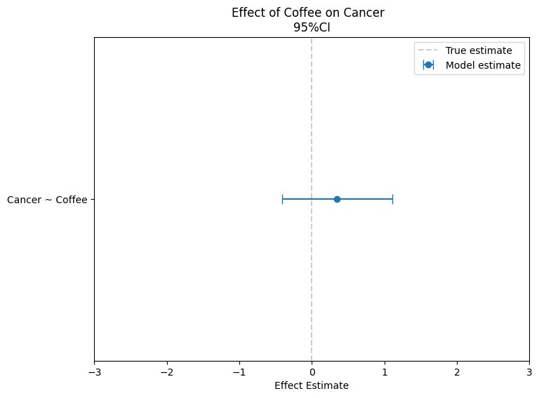
Figure 3: Parameters estimates for Randomized Study

After we run the same regression with randomized data, we find no association between coffee and cancer. This result reflects the true nature of the relationship, as there is no causal link between the two. By using randomization, we have removed the influence of confounders like smoking, ensuring that any observed associations—or lack thereof—are causal. This demonstrates how randomization helps isolate the effect of the treatment, providing a more accurate understanding of cause and effect.

Since the groups are now comparable, the effects we observe are solely due to coffee. Randomization ensures that any differences between the groups are evenly distributed, meaning the observed outcomes can be attributed directly to the effect of coffee alone.But Note that the randomization doesnot gaurantee the balance in the Covariates.See

Isn’t Randomization Magical

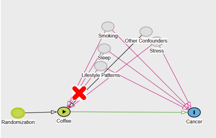
In the coffee example, we only considered one confounder, but in reality, there are often multiple confounders that can complicate the relationship between the exposure (coffee) and the outcome (cancer). These confounders—such as smoking, sleep patterns, stress, and lifestyle choices—can create complex backdoor paths that introduce bias. However, with randomization, we don’t have to worry about these confounders because randomization ensures that they are equally distributed across different treatment groups. This effectively blocks all backdoor paths, allowing us to isolate the true causal effect of the exposure (coffee) on the outcome (cancer).

###TO BE CONTINUED

More on Randomization

Out of Balance, DarrenDahly,PhD

Covariate Adjustment Ewout Steyerbert

statistical Control Requires Causal Justification Wysocki,Lawson,Rhemtulla