Probability Theory Meets Survey Data

Disclaimer: If you notice any similarities with the famous Monty Hall Problem, it’s not just a coincidence. This application was actually inspired by the Monty Hall Problem.

Problem Statement

Imagine you are a skilled statistician overseeing a comprehensive demographic study. Your data collection phase appears to have gone smoothly and you have collected thousands of data, but then you stumble upon a critical revelation. It appears that one of your newly recruited front-line surveyors has unknowingly missed to ask a question from the survey on the back of the last page of the questionnaire. And rather than reporting this oversight to the project lead, the surveyor took it upon themselves to fill in random answer for the missed question which was a choice question.

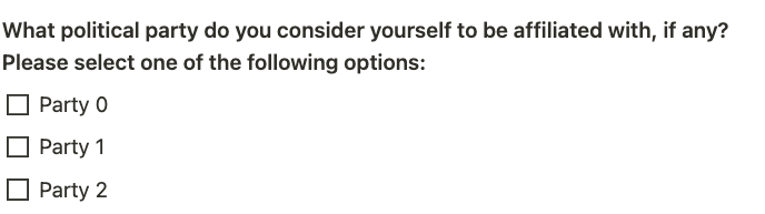
Fig: Sample of that missed question

Now, all the completed questionnaires are mixed in one place, and you are facing the challenge of identifying what proportion of the samples has been affected by this random answering. The gravity of this situation becomes evident as you realize that incorporating this information could significantly impact the accuracy and reliability of your research conclusions.

Objective: identifying what proportion of the samples has been affected

These types issues in surveys are not only common when utilizing human data collectors but can also arise in modern online data collection platforms in which they might be infiltrated with bots. The fact that this information came to light is indeed beneficial, as it enables you to address specific research questions. While this disclosure may influence certain research questions, there are still various aspects we can investigate without incorporating this particular information. However, as a curious statistician, you would be eager to determine the proportion of the sample that provided a random answer to this question.

Probability Theory to the rescue

In our scenario, we have observations of choices denoted as \(X\sim {0, 1, 2}\). However, these observed choices are outcomes of an underlying, hidden process that remains unobserved in other words “Latent”. Nonetheless, these observed data points may offer us insights into the latent variables that generate them. Let’s visualize this system to better understand its dynamics.

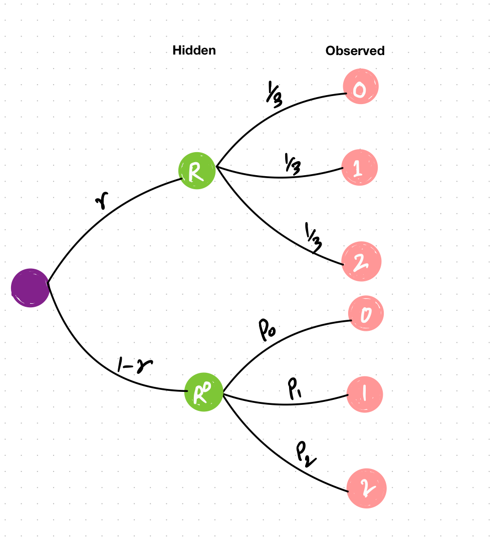
Fig: Probability Tree for given Problem Statement

Here, we have observed variables represented(far-right) which could have been generated from the outcome of a Latent Variable denoted as either randomly answered ($R$) or genuinely answered ($R^0$) with probabilities \(r\) and \((1-r)\) respectively. When the answers are randomly provided, all choices become equally plausible, leading us to assign equal probabilities to each choice i.e \(\frac{1}{3}\). However, if the answers were genuinely provided, we are interested in estimating the proportion of the sample that opted for each choice. These proportions are denoted as p0, p1, and p2 for the observed values 0,1, and 2 respectively which we estimate from the data.

Using Law of Total Probability (LOTP)

\[P(X=0) = p(R) * P(X=0|R) + P(R_{0})*P(X=0|R_{0})\] \[= r *(1/3) + (1-r)*p_{0}\]

Similarly,

\[P(X=1) = r *(1/3) + (1-r)*p_{1}\] \[P(X==2) = = r *(1/3) + (1-r)*p_{2}\]

We are interested in estimating (r), which represents the proportion of samples that were randomly answered. To achieve this estimation, we will employ the Hamiltonian Monte Carlo (HMC) algorithm, an advanced version of the Markov Chain Monte Carlo (MCMC) method. In this process, we will utilize PYMC, a Bayesian library, which eliminates the need to implement HMC manually, streamlining the estimation process

Data Generation

Using simulated data ensures that we have complete knowledge of the true proportion (r), which makes it an ideal testing ground for validating our model and estimation procedure. Once we confirm that our methodology provides reliable estimates, we can confidently apply it to real-world datasets, where the underlying proportions may not be known a priori, and use it to gain valuable insights into latent variables and their impact on observed outcomes.

##
n_sample = 1000
r_real = 0.3
## draw random samples from a bernoulli distribution
R = pm.draw(pm.Bernoulli.dist(r_real),n_sample)

Observed = np.random.choice([0,1,2],size = int(n_sample*r_real))
Observed = np.hstack(
		[
			Observed,
			np.random.choice([0,1,2],p=[0.7,0.2,0.1],size = int(n_sample *(1-r_real)))
     ])

I have generated 1000 samples where 30%(0.3) of the samples were randomly answered (affected).

In probability theory, every unknown parameter gets a prior probability. Here you can also use your information about this if you have some but I am going to use less informative priors for this model pretending I know very less about this variable.

\[X|r=1 \sim Categorical((1/3))\] \[X|r=0 \sim Categorical(p)\] \[r \sim Beta(2,2)\] \[p \sim Dirichlet(2,2,2)\]

import pymc as pm import pytensor.tensor as pt import arviz as az

## Using L.O.T.P from above to compute the likelihood
def logp(value,r,p):
  return at.switch(
      at.eq(value,0),at.logsumexp((at.log(r[0])+at.log(1/3),at.log(r[1])+ at.log(p[0]))),
        at.switch(at.eq(value,1),at.logsumexp((at.log(r[0])+at.log(1/3),at.log(r[1])+at.log(p[1]))),
          at.logsumexp((at.log(r[0])+at.log(1/3),at.log(r[1])+at.log(p[2])))
        )
  )

with pm.Model() as m:
  ## latent variable
  r = pm.Dirichlet("r",(2,2))
  p = pm.Dirichlet("p",[2,2,2])
  pm.DensityDist("LatentMixt", r,p,logp=logp, observed = Observed)
  trace=pm.sample(cores = 2)

az.summary(trace)

| | mean | sd | hdi_3% | hdi_97% | | — | — | — | — | — | | r[0] | 0.28 | 0.109 | 0.089 | 0.473 | | r[1] | 0.71 | 0.109 | 0.527 | 0.911 | | p[0] | 0.70 | 0.057 | 0.608 | 0.813 | | p[1] | 0.20 | 0.028 | 0.149 | 0.253 | | p[2] | 0.09 | 0.036 | 0.032 | 0.161 |

Findings

The results of our analysis demonstrate the effectiveness of our model in estimating the proportion of samples that were randomly filled. In this study, we discovered that approximately 30% (0.30) of the samples were randomly answered of which our model predicted the estimates for (r) with a mean value of about 29% (0.281). This close approximation to the true value confirms the reliability of our methodology.

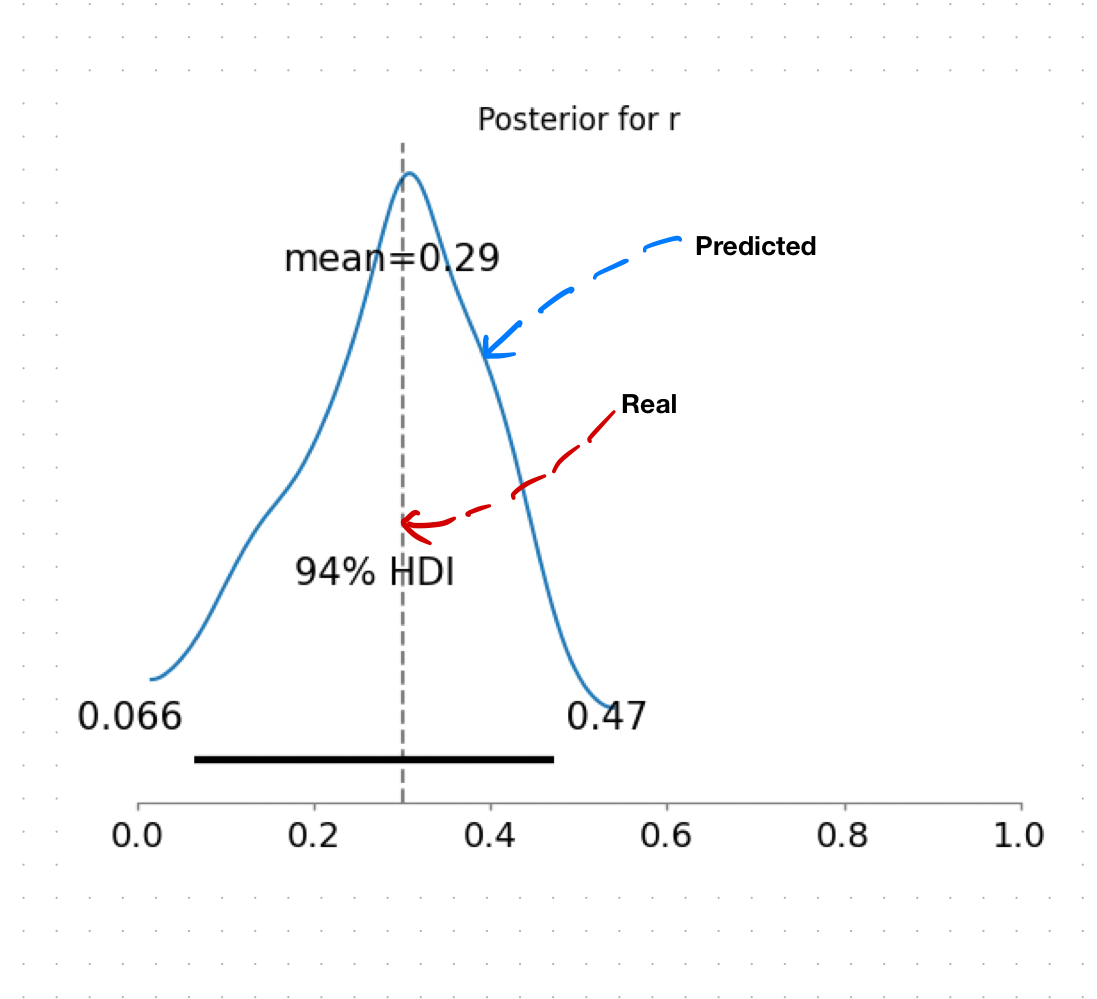
Furthermore, our model provided us with a comprehensive distribution of (r), offering insights into the uncertainty surrounding the estimates. This information proves invaluable in understanding the underlying dynamics and behaviors of the latent variables.

Conclusions

Well, you can play around with these kinds of models which is beyond the scope of this article. However, these findings carry significant implications for survey data analysis and decision-making. Understanding the presence of randomly answered responses allows for more accurate and insightful interpretations of survey results.

Furthermore, You can use these kinds of probabilistic approaches to estimate any kind of underlying latent variables and further use it to answer other research questions without throwing away the data. For example, here we assumed the bots answered the questions randomly; what if the bot is biased? and always selects zero.