Quantifying the Idea of Updating beliefs

Everyone has their go-to example to explain Bayesian Updating. Mine’s just a bit… scary!

Each of us holds a set of beliefs that we have developed through our experiences. Every time we have to make a decision, we tend to base it on those belief i.e. our attitude towards the world at that given time. Although the ability to always search for the motivation to change/update self-beliefs are important for us to make a better decision yet human factors like ego, blind superstition, etc comes as a tyrannical force to prevent us from changing or updating our self-beliefs.

Karl Popper refers to this concept of Idea of Falsification which asserts that science progresses by disproving hypotheses rather than proving them definitively. In line with this, we believe that updating our beliefs in light of new evidence is essential for scientific advancement. For instance, our previous view regarding the form of the Earth was that it was flat, but with the advent of new scientific tools, we can today conclude that it is roughly a sphere. And later we updated our beliefs, and maybe in the future from a different dimension (if exists) Earth’s form can be different from the sphere.

Quantifying and Updating Beliefs (Bayesian formula)

\[P(\theta|evidence)=\frac{P(\theta)*P(evidence|\theta)}{P(evidence)}\]

If you peek at the right side of our equation; this side incorporates both our existing beliefs and the likelihood of the evidence (data); \(P(\theta)\) is our existing belief on \(\theta\) which is called a Prior and P(\(evidence|\theta )\) is our likelihood of the evidence. Thus the left side P( \(\theta| evidence\) )is our updated belief on \(\theta\) . For instance, back to the above analogy; \(\theta\) can be the believed form of the Earth today.

Updating Beliefs about Ghost!! Just a toy example

Scenario

Imagine you’re moving into a new home—this is how the opening scene of many horror films begins. You had some strange experiences and made the decision to keep watch every night for a few days to see what would happen,but how could we reflect these prevailing notions mathematically; Using Bayesian approach, the unknown probability of ghost(p) would be treated as a random variable and given a distribution.Let’s plot some of the Prior beliefs before we discuss its underlying distributions.

Fig 1: Prior Distributions

The above plots are some of our prior distribution which will be explained below, the shaded region indicates that the mass of probability is in that region.

The prior shown in Fig 1 (first from the left), where the shaded region is flat across all values from 0 to 1, suggests a complete lack of prior knowledge or awareness of the phenomenon—almost as if I’m new to the planet, having never heard about ghosts. This first prior is neutral, meaning that all probabilities from 0 to 1 are equally likely. However, we can improve upon this assumption. While ignoring scientific information for the fun of this example, most of us hold certain beliefs shaped by watching countless horror movies or hearing ghost stories from our grandmothers. The rest of the priors reflect that most people hold preconceived beliefs about the existence of ghosts.

The prior shown in Fig 2 (second from the left) suggests that I am more inclined to believe that ghosts don’t exist, though there is still a small chance that they might.

Similarly, Prior from Fig 3 suggests that there is a 50/50 possibility of ghost. The shape of the distribution implies moderate confidence in the 50% belief but doesn’t entirely rule out extreme possibilities.

The prior shown in Fig 4 indicates that I have stronger beliefs in the existence of ghosts, although I still have some uncertainty.

Note: This is just a part of an imaginary exercise; if you are doing a generalizable study you would want to use priors based on some scientific theory or an existing experiment. Or any other priors depending upon the type of your study.

Bayesian Updating

Moving on with “I kind of don’t believe in ghosts”(second from the left). This suggests that the existence of ghosts (p=1) is extremely implausible and the absence of ghosts (p=0) is extremely likely. This does not indicate that there is no chances of ghost,just because the absence of ghosts (p=0) is quite likely. It only suggests that the existence of ghosts (p=1) is exceedingly improbable.

Let’s now enter the monitoring phase and begin gathering and documenting each of our paranormal encounters. Every day is like flipping a coin (Bernoulli trials): if we experience some paranormal activity, we record 1; otherwise, we record 0. See the mathematical instructions at the end of the article.

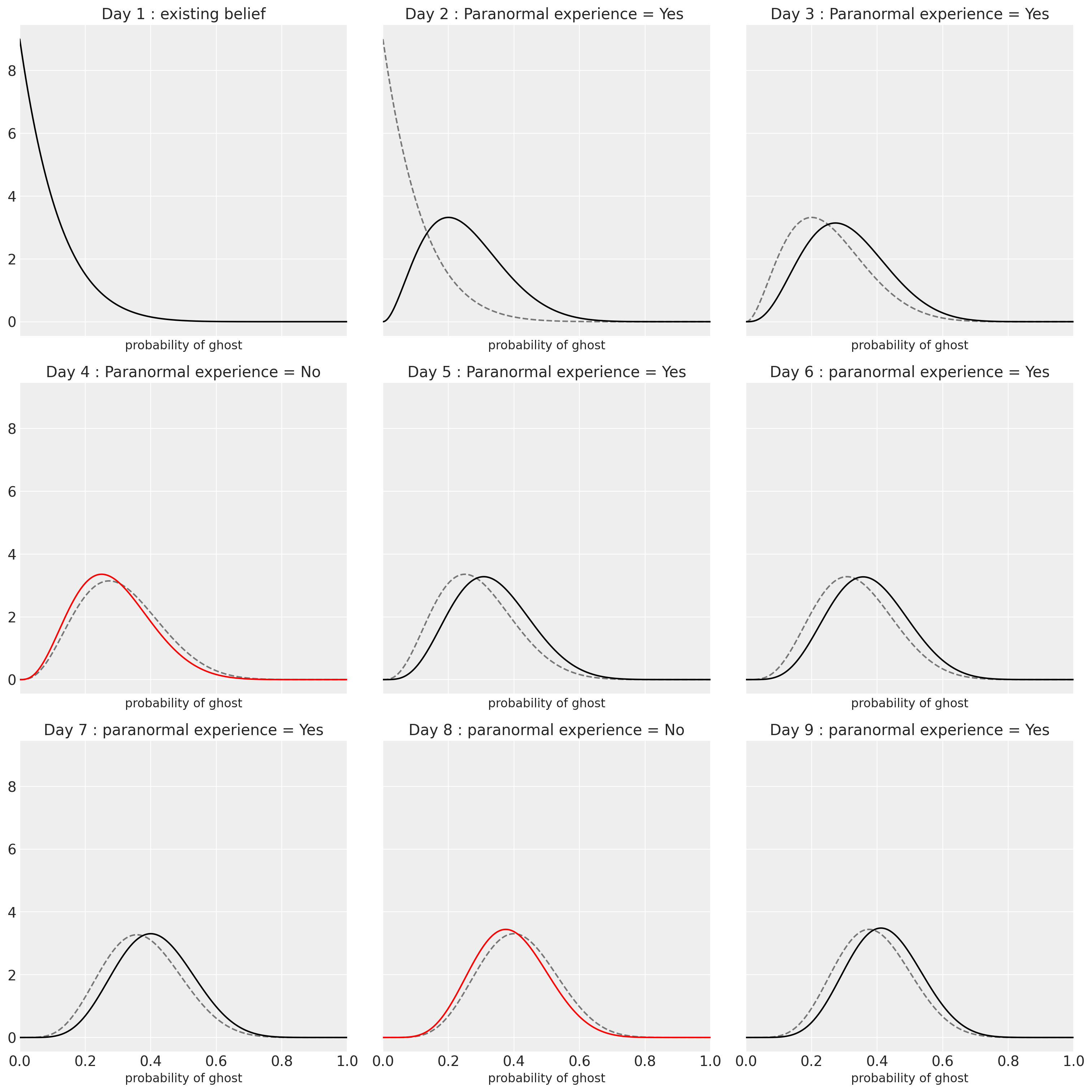
Fig 2: Updating our Beliefs

We begin with our preexisting belief about the ghost; if we have any paranormal experiences, such as discovering someone under the bed, we then shift our beliefs to the right (p=1), but because it is a bayesian shift, we obtain the full distribution. For instance, on Day 2, the dashed distribution represents our prior distribution whereas the solid-line distribution represents our updated belief also as known as Posterior distribution. But an intriguing fact is that we will use this posterior distribution as our prior distribution on day 3 while we monitor the data and revise our opinions.

Change In beliefs

The process of updating continues until day 9, which is the present. Using the same Bayesian formula we previously encountered, we compute our posterior distribution for each day.

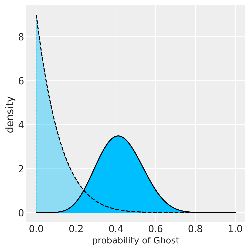
Fig: Updated Beliefs

The black dotted distribution reflects our initial prior belief regarding ghosts; however, the black solid line shows our current beliefs, which lean more toward a 50/50 . Our understanding of the ghost has been updated as a result of our experience, and based on the updated distribution, it appears that it is time to call the priests.

These systems for updating beliefs are hardwired into our brain. This is how we form an opinion on something too, The more strongly we feel about some opinion, the more difficult it is to change our minds. Even though this occurs automatically inside our brains, teaching it to our computers—is a little more tricky. The underlying mathematics are explained next.

Math Section

While there are various methods for computing the posterior distribution (updated belief), they fundamentally rely on the Bayesian formula we discussed earlier. Some of these approaches include sampling, analytical solutions, and quadratic approximations. In this case, we are calculating the posterior, or updated beliefs, using an analytical solution (Beta-Bernoulli Conjugacy). Although this method is less commonly used today, it is particularly well-suited for illustrating the example at hand.

Since everything that can be expressed mathematically can be coded into computers, we will attempt to express our beliefs through mathematical expressions.

Beta-Bernoulli conjugacy

Using the Bayesian Formula;

\[P(\theta|X)=\frac{P(\theta)*P(X|\theta)}{P(\theta)} \quad \quad \quad \text{[X here is observed data]}\]

We are interested in

\[P(\theta|X)\]

which is our posterior distribution i.e probability of ghost(\(\theta\)) given the data (X) where X can take value either 0 or 1.

Defining our Prior and Likelihoods:

\[P(\theta)\sim Beta(\alpha,\beta) \quad \quad \quad \text{[Prior]}\] \[\theta \sim \frac{\theta^{\alpha-1} *(1-\theta)^{\beta-1}}{B(\alpha,\beta)}\]

\(B(\alpha,\beta)\) is a constant and it does not depend on \(\theta\) we can remove it from the equation

\[f(\theta) = {\theta^{\alpha-1} *(1-\theta)^{\beta-1}}\]

Now we define our likelihood; where X is the random Variable that can take values X can take values either of {0,1}.

\[P(X|\theta) \sim Bernoulli(\theta) \quad \quad \quad \text{[ Bernoulli likelihood]}\] \[P(X|\theta) \sim \theta^{x} (1-\theta)^{1-x}\]

Since, we have everything we need; plugging the values in above formula;

\[P(\theta|X)=\frac{P(\theta)*P(X|\theta)}{P(\theta)}\] \[P(\theta|X)= \theta^{(\alpha + x)-1} (1-\theta)^{(\beta-x)-1}\]

let,\(\alpha'=\alpha + k\) and \(\beta'=\beta-k\);

\[P(\theta|X)= \theta^{\alpha'} (1-\theta)^{(\beta+n-x)-1}\]

using proportionality of equations

\[P(\theta|X) = \frac{\theta^{(\alpha + x)-1} (1-\theta)^{(\beta+n-x)-1}}{B(\alpha',\beta')} \quad \quad \quad \text{[Updated Belief]}\] \[P(\theta|X) =Beta(\alpha',\beta') \quad \quad \quad \text{[which is also a Beta Distribution]}\]