Multilevel Models and Causal Dilemmas
Context
Multilevel models are powerful—but they can silently mislead you. A single overlooked assumption can flip your causal conclusions upside down. Many analysts unknowingly violate a key assumption: that predictors must be uncorrelated with group-level error terms (Antonakis et al., 2019). When this assumption is violated, endogeneity arises, leading to biased and misleading causal estimates.
In this post, we explore:
- Why and when this endogeneity creeps into multilevel models
- How Mundlak adjustments and contextual variables help address the bias
- How to causally interpret these contextual effects
To bring these ideas to life, we’ll simulate a realistic marketing scenario where we estimate how regional ad spend affects profit—and show how different modeling choices can lead to dramatically different conclusions. (Code will be provided in the Appendix below)
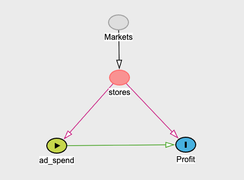
Figure: Directed Acyclic Graph (DAG) showing the data generation process. Regional competition influences both average ad spend and profit, creating confounding that must be properly controlled for in causal analysis.
We simulate monthly profit reports for businesses operating across \(R = n_{\text{regions}}\) regions. Each region \(r \in \{1, \dots, R\}\) has a latent competition score:
\[C_r \sim \mathcal{N}(0, 10^2)\]This competition score influences regional-level advertising spend, such that:
\[\text{AdSpend}^{\text{avg}}_r \sim \mathcal{N}(2 \cdot C_r, 2^2)\]Each region produces a varying number of monthly reports (because not all stores were set up at the same time, but we take regions that have at least 2 months of data):
\[T_r \sim \text{Poisson}(5) + 2\]At the individual (monthly) level, we simulate ad spend with individual noise:
\[\text{AdSpend}_{it} \sim \mathcal{N}(\text{AdSpend}^{\text{avg}}_r, 5^2)\]Finally, profit is generated based on:
- A baseline value of 8
- A negative effect of competition with weight \(-3.0\)
- A positive effect of ad spend with coefficient \(\beta = 1.5\)
This setup results in hierarchical data with both region-level structure and individual-level variation, making it ideal for evaluating multilevel modeling techniques.
Data Visualization
The plot of the data for \(n_{\text{region}} = 10\) is shown below:
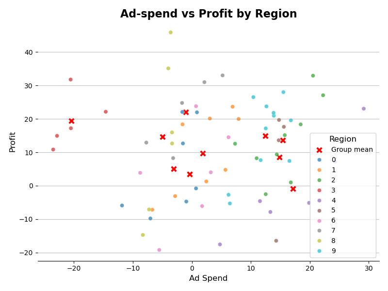
Figure: Ad spend vs. Profit by regions
At first glance, it appears that ad spend is not generating profits. However, our research objective is not to look at the overall effect (which has no causal interpretation and no actionable properties), but rather to examine the within-region effects. This is why it is necessary to stratify by regions and why drawing a DAG is useful.
The Random Effects Model (Biased)
To account for unobserved heterogeneity across regions, a common approach is to use fixed effects models, but I have started with a dummy-variable model. This setup is equivalent to a fixed effects model with dummy variables for each region. Here, we estimate a separate intercept \(\alpha_{r}\) per region, which controls for all time-invariant regional confounders.
\[\text{Profit}_{rt} \sim \mathcal{N}(\alpha_{r} + \beta \cdot \text{AdSpend}_{rt}, \sigma)\]But to reap the benefits of hierarchical modeling, analysts often switch to random effects models with random intercepts. So you would usually just add one more prior on level 2 (region) without explicitly checking the assumptions of RE models. This is where potentially the assumptions are missed.
\[\text{Profit}_{rt} \sim \mathcal{N}(\alpha_{r} + \beta \cdot \text{AdSpend}_{rt}, \sigma)\] \[\alpha_{r} \sim \mathcal{N}(\mu_a, \sigma_{a})\]Here, the region-specific intercepts \(\alpha_r\) are drawn from a common distribution, introducing partial pooling: This improves estimates in regions with limited data and allows for generalization beyond observed regions.
However, this model relies on a crucial assumption:
The predictor \(\text{AdSpend}_{rt}\) must be uncorrelated with the group-level error component \(\sigma_a\) for the causal estimates of the within effects to be true.
If this assumption is violated—say, because an unobserved confounder like regional competition influences both ad spend and profit—then endogeneity arises. In that case, the estimated within-effects \(\beta\) will be biased, even though the model appears statistically sound.
This problem is illustrated in the figure below:
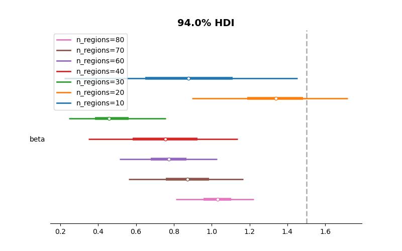
Figure: Posterior estimates (94% HDI) of \(\beta\) across different numbers of regions. The dashed line indicates the true value. The random effects model systematically underestimates the true effect due to unaccounted confounding
Because this is a simulated dataset, this gives us the luxury of knowing what the correct answer should be, and the model fit does not give us the right answer at different levels of analysis. Here the true parameter is 1.5 and the model fails to recover the right estimates under different numbers of regions in this hypothetical simulated case.
The Mundlak-Style Random Effects Model
Now let’s introduce the Mundlak-style random effects model:
\[\text{Profit}_{rt} \sim \mathcal{N}(\alpha_{r} + \beta \cdot \text{AdSpend}_{rt} + \beta_{1} \cdot \overline{\text{AdSpend}}_r, \sigma)\] \[\alpha_{r} \sim \mathcal{N}(\mu_a, \sigma_{a})\]The only visible difference here is that the model gets a \(\beta_{1} \cdot \overline{\text{AdSpend}}\) term in the model. The parameter \(\beta_1\) here is also called Mundlak adjustment and gives you the contextual effect in this case.
Now let’s compare these model fits side by side:
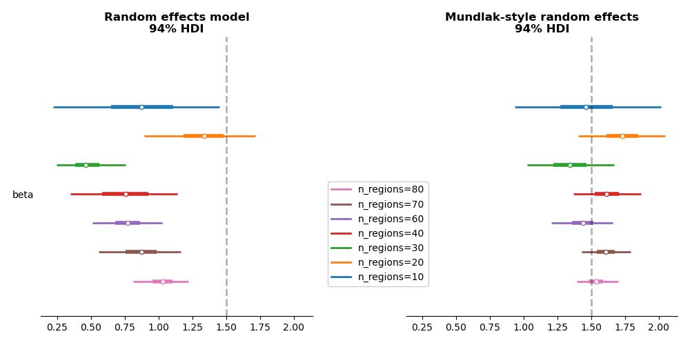
Figure: Comparison of model estimates. The naive random effects model (left) underestimates the true effect due to confounding. The Mundlak-style model (right) correctly identifies the causal effect of ad spend on profit.
By correcting the model in this way, we recover estimates that are both more accurate and causally interpretable.
Understanding Endogeneity
This bias occurs because endogeneity arises when a regressor is correlated with the level 2 error term in a regression model, i.e., \(\text{Cov}(\text{AdSpend}_{rt}, \sigma_a) \neq 0\).
Yes — I’ve repeated this assumption multiple times throughout the post, and that’s intentional. It’s absolutely fundamental. Ignoring it introduces bias that can completely distort your causal conclusions.
In classical (frequentist) statistics, the Hausman test is often used to detect such violations by comparing fixed and random effects estimates. But in a Bayesian framework, we can inspect the posterior samples directly to diagnose the problem.
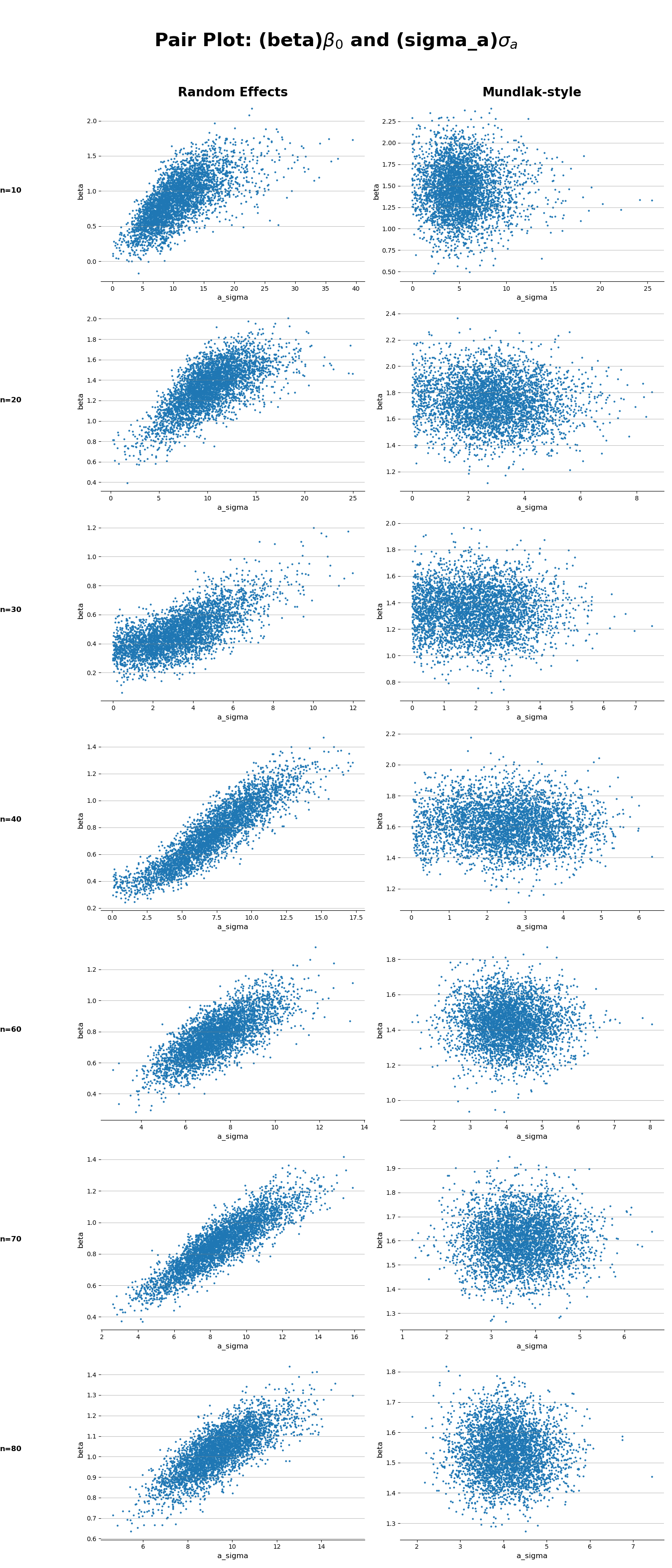
In the naive model (left), the strong posterior correlation between the slope
\(\beta\) and the level 2 error term \(\sigma_{a}\) is a red flag: the model hasn’t separated within-region and between-region variation. In contrast, the Mundlak-adjusted model (right) shows much cleaner, uncorrelated posteriors—suggesting that the contextual adjustment successfully removed the bias.
Interpreting Contextual Effects
Another important aspect of Mundlak-style multilevel regression is the interpretation of contextual effects. This might be a bit tricky because the effect of ad-spend (\(\beta\)) is positive, but if you look at the model summary for each simulation (code in the Appendix) the effect of average ad-spend (\(\beta_1\)) is negative. What would this mean?
The parameter \(\beta_1\) should not be interpreted as a within-effect, but rather, many regions’ average ad spend are proxies that tell us about their underlying causes—in this case, competition. Here we generated the dataset ourselves, we know this relationship exists. However, this is not always this easy to interpret and does not always have a causal interpretation, so it should be interpreted carefully.
The contextual effect (\(\beta_1\)) reflects the difference between the total (marginal) effect of ad spend across regions and the within-region effect (\(\beta\)). It captures how much of the ad spend’s apparent effect is explained by group-level (between-region) differences.
Appendix
Analysis Notebook, containing simulations and models
On Ignoring the Random Effects Assumption in Multilevel Models: Review, Critique, and Recommendations, Antonakis, J., Bastardoz, N., & Rönkkö, M. (2019)